pacman::p_load(tmap, sf, sp, DT,
               performance, reshape2,
ggpubr, units, tidyverse)In-class Exercise 3 - Calibrating Spatial Interaction Models with R
Overview
This in-class introduces an alternative R package to spdep package you used in Hands-on Exercise 6. The package is called sfdep. According to Josiah Parry, the developer of the package, “sfdep builds on the great shoulders of spdep package for spatial dependence. sfdep creates an sf and tidyverse friendly interface to the package as well as introduces new functionality that is not present in spdep. sfdep utilizes list columns extensively to make this interface possible.”
Getting started
mpsz <- st_read(dsn = "data/geospatial",
                   layer = "MPSZ-2019") %>%
  st_transform(crs = 3414)
Reading layer `MPSZ-2019' from data source
`C:\weipengten\ISSS624\In-class_Ex\In-class_Ex3\data\geospatial'
using driver `ESRI Shapefile'
Simple feature collection with 332 features and 6 fields
Geometry type: MULTIPOLYGON
Dimension: XY
Bounding box: xmin: 103.6057 ymin: 1.158699 xmax: 104.0885 ymax: 1.470775
Geodetic CRS: WGS 84mpsz_sp <- as(mpsz, "Spatial")
mpsz_spclass : SpatialPolygonsDataFrame
features : 332
extent : 2667.538, 56396.44, 15748.72, 50256.33 (xmin, xmax, ymin, ymax)
crs : +proj=tmerc +lat_0=1.36666666666667 +lon_0=103.833333333333 +k=1 +x_0=28001.642 +y_0=38744.572 +ellps=WGS84 +towgs84=0,0,0,0,0,0,0 +units=m +no_defs
variables : 6
names : SUBZONE_N, SUBZONE_C, PLN_AREA_N, PLN_AREA_C, REGION_N, REGION_C
min values : ADMIRALTY, AMSZ01, ANG MO KIO, AM, CENTRAL REGION, CR
max values : YUNNAN, YSSZ09, YISHUN, YS, WEST REGION, WR dist <- spDists(mpsz_sp,
longlat = FALSE)
head(dist, n=c(10, 10)) [,1] [,2] [,3] [,4] [,5] [,6] [,7]
[1,] 0.000 3926.0025 3939.108 20252.964 2989.9839 1431.330 19211.836
[2,] 3926.003 0.0000 305.737 16513.865 951.8314 5254.066 16242.523
[3,] 3939.108 305.7370 0.000 16412.062 1045.9088 5299.849 16026.146
[4,] 20252.964 16513.8648 16412.062 0.000 17450.3044 21665.795 7229.017
[5,] 2989.984 951.8314 1045.909 17450.304 0.0000 4303.232 17020.916
[6,] 1431.330 5254.0664 5299.849 21665.795 4303.2323 0.000 20617.082
[7,] 19211.836 16242.5230 16026.146 7229.017 17020.9161 20617.082 0.000
[8,] 14960.942 12749.4101 12477.871 11284.279 13336.0421 16281.453 5606.082
[9,] 7515.256 7934.8082 7649.776 18427.503 7801.6163 8403.896 14810.930
[10,] 6391.342 4975.0021 4669.295 15469.566 5226.8731 7707.091 13111.391
[,8] [,9] [,10]
[1,] 14960.942 7515.256 6391.342
[2,] 12749.410 7934.808 4975.002
[3,] 12477.871 7649.776 4669.295
[4,] 11284.279 18427.503 15469.566
[5,] 13336.042 7801.616 5226.873
[6,] 16281.453 8403.896 7707.091
[7,] 5606.082 14810.930 13111.391
[8,] 0.000 9472.024 8575.490
[9,] 9472.024 0.000 3780.800
[10,] 8575.490 3780.800 0.00016.5.3 Labelling column and row heanders of a distance matrix
sz_names <- mpsz$SUBZONE_C
colnames(dist) <- paste0(sz_names)
rownames(dist) <- paste0(sz_names)
distPair <- melt(dist) %>%
rename(dist = value)
head(distPair, 10) Var1 Var2 dist
1 MESZ01 MESZ01 0.000
2 RVSZ05 MESZ01 3926.003
3 SRSZ01 MESZ01 3939.108
4 WISZ01 MESZ01 20252.964
5 MUSZ02 MESZ01 2989.984
6 MPSZ05 MESZ01 1431.330
7 WISZ03 MESZ01 19211.836
8 WISZ02 MESZ01 14960.942
9 SISZ02 MESZ01 7515.256
10 SISZ01 MESZ01 6391.34216.5.5 Updating intra-zonal distances
In this section, we are going to append a constant value to replace the intra-zonal distance of 0.
First, we will select and find out the minimum value of the distance by using summary().
distPair %>%
  filter(dist > 0) %>%
  summary()
Var1 Var2 dist
MESZ01 : 331 MESZ01 : 331 Min. : 173.8
RVSZ05 : 331 RVSZ05 : 331 1st Qu.: 7149.5
SRSZ01 : 331 SRSZ01 : 331 Median :11890.0
WISZ01 : 331 WISZ01 : 331 Mean :12229.4
MUSZ02 : 331 MUSZ02 : 331 3rd Qu.:16401.7
MPSZ05 : 331 MPSZ05 : 331 Max. :49894.4
(Other):107906 (Other):107906 Next, a constant distance value of 50m is added into intra-zones distance. > 50 is derived from approximately minimum of 173.8 (found out earlier in summary statistics) divided by 2. Note : *Intra-zone
distPair$dist <- ifelse(distPair$dist == 0,
                        50, distPair$dist)
distPair %>%
  summary()
Var1 Var2 dist
MESZ01 : 332 MESZ01 : 332 Min. : 50
RVSZ05 : 332 RVSZ05 : 332 1st Qu.: 7097
SRSZ01 : 332 SRSZ01 : 332 Median :11864
WISZ01 : 332 WISZ01 : 332 Mean :12193
MUSZ02 : 332 MUSZ02 : 332 3rd Qu.:16388
MPSZ05 : 332 MPSZ05 : 332 Max. :49894
(Other):108232 (Other):108232 distPair <- distPair %>%
rename(orig = Var1,
dest = Var2)
write_rds(distPair, "data/rds/distPair.rds") 16.6 Preparing flow data
od_data <- read_rds("data/rds/od_data.rds")

flow_data <- od_data %>%
  group_by(ORIGIN_SZ, DESTIN_SZ) %>%
  summarize(TRIPS = sum(MORNING_PEAK))

head(flow_data, 10)
# A tibble: 10 × 3
# Groups: ORIGIN_SZ [1]
ORIGIN_SZ DESTIN_SZ TRIPS
<chr> <chr> <dbl>
1 AMSZ01 AMSZ01 2694
2 AMSZ01 AMSZ02 10591
3 AMSZ01 AMSZ03 14980
4 AMSZ01 AMSZ04 3106
5 AMSZ01 AMSZ05 7734
6 AMSZ01 AMSZ06 2306
7 AMSZ01 AMSZ07 1824
8 AMSZ01 AMSZ08 2734
9 AMSZ01 AMSZ09 2300
10 AMSZ01 AMSZ10 16416.6.1 Separating intra-flow from passenger volume df
flow_data$FlowNoIntra <- ifelse(
  flow_data$ORIGIN_SZ == flow_data$DESTIN_SZ,
  0, flow_data$TRIPS)
flow_data$offset <- ifelse(
  flow_data$ORIGIN_SZ == flow_data$DESTIN_SZ,
  0.000001, 1)
16.6.2 Combining passenger volume data with distance value
Before we can join flow_data and distPair, we need to convert data value type of ORIGIN_SZ and DESTIN_SZ fields of flow_data dataframe into factor data type.
flow_data$ORIGIN_SZ <- as.factor(flow_data$ORIGIN_SZ)
flow_data$DESTIN_SZ <- as.factor(flow_data$DESTIN_SZ)
Now, left_join() of dplyr will be used to merge flow_data dataframe and distPair dataframe. The output is called flow_data1.
flow_data1 <- flow_data %>%
  left_join (distPair,
             by = c("ORIGIN_SZ" = "orig",
                    "DESTIN_SZ" = "dest"))
16.7 Preparing Origin and Destination Attributes
16.7.1 Importing population data
pop <- read_csv("data/aspatial/pop.csv")16.7.2 Geospatial data wrangling
pop <- pop %>%
  left_join(mpsz,
            by = c("PA" = "PLN_AREA_N",
                   "SZ" = "SUBZONE_N")) %>%
  select(1:6, everything()) %>%
  rename(SZ_NAME = SZ,
         SZ = SUBZONE_C)
16.7.3 Preparing origin attribute
flow_data1 <- flow_data1 %>%
  left_join(pop,
            by = c(ORIGIN_SZ = "SZ")) %>%
  rename(ORIGIN_AGE7_12 = AGE7_12,
         ORIGIN_AGE13_24 = AGE13_24,
         ORIGIN_AGE25_64 = AGE25_64) %>%
  select(-c(PA, SZ_NAME))
16.7.4 Preparing destination attribute
flow_data1 <- flow_data1 %>%
  left_join(pop,
            by = c(DESTIN_SZ = "SZ")) %>%
  select(-c(PA, SZ_NAME)) %>%
  rename(DESTIN_AGE7_12 = AGE7_12,
         DESTIN_AGE13_24 = AGE13_24,
         DESTIN_AGE25_64 = AGE25_64)

write_rds(flow_data1, "data/rds/SIM_data")
16.8 Calibrating Spatial Interaction Models
In this section, you will learn how to calibrate Spatial Interaction Models by using Poisson Regression method.
16.8.1 Importing the modelling data
Firstly, let us import the modelling data by using the code chunk below.
SIM_data <- read_rds("data/rds/SIM_data.rds")16.8.2 Visualising the dependent variable
Firstly, let us plot the distribution of the dependent variable (i.e. TRIPS) by using histogram method by using the code chunk below.
ggplot(data = SIM_data,
       aes(x = TRIPS)) +
  geom_histogram()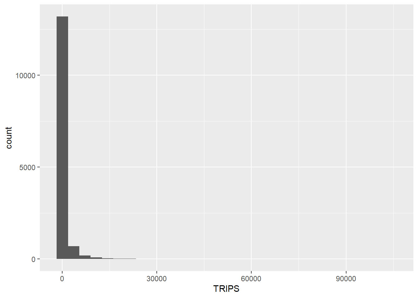
Notice that the distribution is highly skewed and not resemble bell shape or also known as normal distribution.
Next, let us visualise the relation between the dependent variable and one of the key independent variable in Spatial Interaction Model, namely distance.
ggplot(data = SIM_data,
       aes(x = dist,
           y = TRIPS)) +
  geom_point() +
  geom_smooth(method = lm)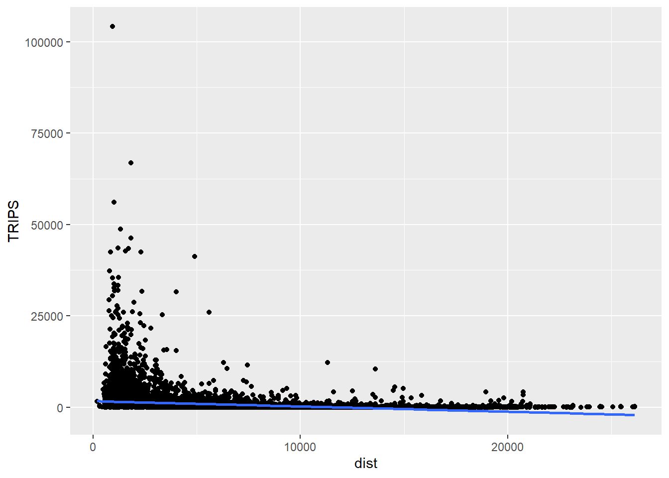
Notice that their relationship hardly resemble linear relationship.
On the other hand, if we plot the scatter plot by using the log transformed version of both variables, we can see that their relationship is more resemble linear relationship.
ggplot(data = SIM_data,
       aes(x = log(dist),
           y = log(TRIPS))) +
  geom_point() +
  geom_smooth(method = lm)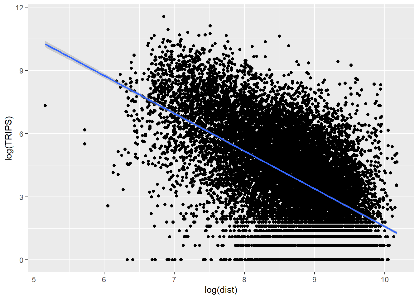
16.8.3 Checking for variables with zero values
Since Poisson Regression is based of log and log 0 is undefined, it is important for us to ensure that no 0 values in the explanatory variables.
In the code chunk below, summary() of Base R is used to compute the summary statistics of all variables in SIM_data data frame.
summary(SIM_data) ORIGIN_SZ DESTIN_SZ TRIPS FlowNoIntra
Length:14274 Length:14274 Min. : 1.0 Min. : 1.0
Class :character Class :character 1st Qu.: 11.0 1st Qu.: 11.0
Mode :character Mode :character Median : 56.0 Median : 56.0
Mean : 664.3 Mean : 664.3
3rd Qu.: 296.0 3rd Qu.: 296.0
Max. :104167.0 Max. :104167.0
offset dist ORIGIN_AGE7_12 ORIGIN_AGE13_24 ORIGIN_AGE25_64
Min. :1 Min. : 173.8 Min. : 0 Min. : 0 Min. : 0
1st Qu.:1 1st Qu.: 3465.4 1st Qu.: 240 1st Qu.: 460 1st Qu.: 2210
Median :1 Median : 6121.0 Median : 710 Median : 1400 Median : 7030
Mean :1 Mean : 6951.8 Mean :1037 Mean : 2278 Mean :10536
3rd Qu.:1 3rd Qu.: 9725.1 3rd Qu.:1500 3rd Qu.: 3282 3rd Qu.:15830
Max. :1 Max. :26135.8 Max. :6340 Max. :16380 Max. :74610
DESTIN_AGE7_12 DESTIN_AGE13_24 DESTIN_AGE25_64
Min. : 0 Min. : 0 Min. : 0
1st Qu.: 250 1st Qu.: 460 1st Qu.: 2210
Median : 720 Median : 1430 Median : 7120
Mean :1040 Mean : 2305 Mean :10648
3rd Qu.:1500 3rd Qu.: 3290 3rd Qu.:15830
Max. :6340 Max. :16380 Max. :74610 The print report above reveals that variables ORIGIN_AGE7_12, ORIGIN_AGE13_24, ORIGIN_AGE25_64,DESTIN_AGE7_12, DESTIN_AGE13_24, DESTIN_AGE25_64 consist of 0 values.
In view of this, code chunk below will be used to replace zero values to 0.99.
SIM_data$DESTIN_AGE7_12 <- ifelse(
  SIM_data$DESTIN_AGE7_12 == 0,
  0.99, SIM_data$DESTIN_AGE7_12)
SIM_data$DESTIN_AGE13_24 <- ifelse(
  SIM_data$DESTIN_AGE13_24 == 0,
  0.99, SIM_data$DESTIN_AGE13_24)
SIM_data$DESTIN_AGE25_64 <- ifelse(
  SIM_data$DESTIN_AGE25_64 == 0,
  0.99, SIM_data$DESTIN_AGE25_64)
SIM_data$ORIGIN_AGE7_12 <- ifelse(
  SIM_data$ORIGIN_AGE7_12 == 0,
  0.99, SIM_data$ORIGIN_AGE7_12)
SIM_data$ORIGIN_AGE13_24 <- ifelse(
  SIM_data$ORIGIN_AGE13_24 == 0,
  0.99, SIM_data$ORIGIN_AGE13_24)
SIM_data$ORIGIN_AGE25_64 <- ifelse(
  SIM_data$ORIGIN_AGE25_64 == 0,
  0.99, SIM_data$ORIGIN_AGE25_64)
Notice that all the 0 values have been replaced by 0.99.
16.8.4 Unconstrained Spatial Interaction Model
In this section, you will learn how to calibrate an unconstrained spatial interaction model by using glm() of Base Stats. The explanatory variables are origin population by different age cohort, destination population by different age cohort (i.e. ORIGIN_AGE25_64) and distance between origin and destination in km (i.e. dist).
The general formula of Unconstrained Spatial Interaction Model
uncSIM <- glm(formula = TRIPS ~
                log(ORIGIN_AGE25_64) +
                log(DESTIN_AGE25_64) +
                log(dist),
              family = poisson(link = "log"),
              data = SIM_data,
              na.action = na.exclude)
uncSIM
Call:  glm(formula = TRIPS ~ log(ORIGIN_AGE25_64) + log(DESTIN_AGE25_64) +
    log(dist), family = poisson(link = "log"), data = SIM_data,
    na.action = na.exclude)

Coefficients:
         (Intercept)  log(ORIGIN_AGE25_64)  log(DESTIN_AGE25_64)
            17.00287               0.21001               0.01289
           log(dist)
            -1.51785

Degrees of Freedom: 14273 Total (i.e. Null);  14270 Residual
Null Deviance:      36120000
Residual Deviance: 19960000     AIC: 20040000
16.8.5 R-squared function
In order to measure how much variation of the trips can be accounted by the model we will write a function to calculate R-Squared value as shown below.
CalcRSquared <- function(observed,estimated){
  r <- cor(observed,estimated)
  R2 <- r^2
  R2
}
Next, we will compute the R-squared of the unconstrained SIM by using the code chunk below.
CalcRSquared(uncSIM$data$TRIPS, uncSIM$fitted.values)[1] 0.1694734r2_mcfadden(uncSIM)# R2 for Generalized Linear Regression
R2: 0.446
adj. R2: 0.44616.8.6 Origin (Production) constrained SIM
In this section, we will fit an origin constrained SIM by using the code3 chunk below.
The general formula of Origin Constrained Spatial Interaction Model
orcSIM <- glm(formula = TRIPS ~
                 ORIGIN_SZ +
                 log(DESTIN_AGE25_64) +
                 log(dist),
              family = poisson(link = "log"),
              data = SIM_data,
              na.action = na.exclude)
We can examine how the constraints hold for destinations this time.
CalcRSquared(orcSIM$data$TRIPS, orcSIM$fitted.values)[1] 0.402911516.8.7 Destination constrained
In this section, we will fit a destination constrained SIM by using the code chunk below.
decSIM <- glm(formula = TRIPS ~
                DESTIN_SZ +
                log(ORIGIN_AGE25_64) +
                log(dist),
              family = poisson(link = "log"),
              data = SIM_data,
              na.action = na.exclude)
We can examine how the constraints hold for destinations this time.
CalcRSquared(decSIM$data$TRIPS, decSIM$fitted.values)[1] 0.49616616.8.8 Doubly constrained
In this section, we will fit a doubly constrained SIM by using the code chunk below.
dbcSIM <- glm(formula = TRIPS ~
                ORIGIN_SZ +
                DESTIN_SZ +
                log(dist),
              family = poisson(link = "log"),
              data = SIM_data,
              na.action = na.exclude)
We can examine how the constraints hold for destinations this time.
CalcRSquared(dbcSIM$data$TRIPS, dbcSIM$fitted.values)[1] 0.6883675Notice that there is a relatively greater improvement in the R^2 value.
16.8.9 Model comparison
Another useful model performance measure for continuous dependent variable is Root Mean Squared Error. In this sub-section, you will learn how to use compare_performance() of performance package
First of all, let us create a list called model_list by using the code chunk below.
model_list <- list(unconstrained=uncSIM,
                   originConstrained=orcSIM,
                   destinationConstrained=decSIM,
                   doublyConstrained=dbcSIM)
Next, we will compute the RMSE of all the models in model_list file by using the code chunk below.
compare_performance(model_list,
                    metrics = "RMSE")
# Comparison of Model Performance Indices
Name | Model | RMSE
-----------------------------------------
unconstrained | glm | 2429.978
originConstrained | glm | 2057.579
destinationConstrained | glm | 1891.724
doublyConstrained | glm | 1487.111The print above reveals that doubly constrained SIM is the best model among all the four SIMs because it has the smallest RMSE value of 1487.111.
16.8.10 Visualising fitted
In this section, you will learn how to visualise the observed values and the fitted values.
Firstly we will extract the fitted values from each model by using the code chunk below.
df <- as.data.frame(uncSIM$fitted.values) %>%
  round(digits = 0)
Next, we will join the values to SIM_data data frame.
SIM_data <- SIM_data %>%
  cbind(df) %>%
  rename(uncTRIPS = "uncSIM$fitted.values")
Repeat the same step by for Origin Constrained SIM (i.e. orcSIM)
df <- as.data.frame(orcSIM$fitted.values) %>%
  round(digits = 0)

SIM_data <- SIM_data %>%
  cbind(df) %>%
  rename(orcTRIPS = "orcSIM$fitted.values")
Repeat the same step by for Destination Constrained SIM (i.e. decSIM)
df <- as.data.frame(decSIM$fitted.values) %>%
  round(digits = 0)
Repeat the same step by for Doubly Constrained SIM (i.e. dbcSIM)
df <- as.data.frame(dbcSIM$fitted.values) %>%
  round(digits = 0)

SIM_data <- SIM_data %>%
  cbind(df) %>%
  rename(dbcTRIPS = "dbcSIM$fitted.values")
unc_p <- ggplot(data = SIM_data,
                aes(x = uncTRIPS,
                    y = TRIPS)) +
  geom_point() +
  geom_smooth(method = lm)

orc_p <- ggplot(data = SIM_data,
                aes(x = orcTRIPS,
                    y = TRIPS)) +
  geom_point() +
  geom_smooth(method = lm)


dec_p <- ggplot(data = SIM_data,
                aes(x = decTRIPS,
                    y = TRIPS)) +
  geom_point() +
  geom_smooth(method = lm)

dbc_p <- ggplot(data = SIM_data,
                aes(x = dbcTRIPS,
                    y = TRIPS)) +
  geom_point() +
  geom_smooth(method = lm)