pacman::p_load(tmap, sf, tidyverse,
knitr)In-class Exercise 1: My First Date with Geospatial Data Science
The Task
In this in-class exercise, you are required to prepare a choropleth map showing the distribution of passenger trips at planning sub-zone by integrating Passenger Volume by Origin Destination Bus Stops and bus stop data sets downloaded from LTA DataMall and Planning Sub-zone boundary of URA Master Plan 2019 downloaded from data.gov.sg.

The specific task of this in-class exercise are as follows:
- to import Passenger Volume by Origin Destination Bus Stops data set downloaded from LTA DataMall in to RStudio environment,
- to import geospatial data in ESRI shapefile format into sf data frame format,
- to perform data wrangling by using appropriate functions from tidyverse and sf pakcges, and
- to visualise the distribution of passenger trip by using tmap methods and functions.
Getting Started
Three R packages will be used in this in-class exercise, they are:
- tidyverse for non-spatial data handling,
- sf for geospatial data handling,
- tmap for thematic mapping, and
- knitr for creating html table.
Using the steps you learned from Hands-on Exercise 1, load these three R packages into RStudio.
Importing the OD data
Firstly, we will import the Passenger Volume by Origin Destination Bus Stops data set downloaded from LTA DataMall by using read_csv() of readr package.
Using the steps you learned from Hands-on Exercise 1, import origin_destination_bus_202308.csv downloaded from LTA DataMall into RStudio and save it as a tibble data frame called odbus.
odbus <- read_csv("data/aspatial/origin_destination_bus_202308.csv")A quick check of odbus tibble data frame shows that the values in OROGIN_PT_CODE and DESTINATON_PT_CODE are in numeric data type.
glimpse(odbus)Rows: 5,709,512
Columns: 7
$ YEAR_MONTH <chr> "2023-08", "2023-08", "2023-08", "2023-08", "2023-…
$ DAY_TYPE <chr> "WEEKDAY", "WEEKENDS/HOLIDAY", "WEEKENDS/HOLIDAY",…
$ TIME_PER_HOUR <dbl> 16, 16, 14, 14, 17, 17, 17, 17, 7, 17, 14, 10, 10,…
$ PT_TYPE <chr> "BUS", "BUS", "BUS", "BUS", "BUS", "BUS", "BUS", "…
$ ORIGIN_PT_CODE <chr> "04168", "04168", "80119", "80119", "44069", "4406…
$ DESTINATION_PT_CODE <chr> "10051", "10051", "90079", "90079", "17229", "1722…
$ TOTAL_TRIPS <dbl> 7, 2, 3, 10, 5, 4, 3, 22, 3, 3, 7, 1, 3, 1, 3, 1, …Using appropriate tidyverse functions to convert these data values into factor data type.
odbus$ORIGIN_PT_CODE <- as.factor(odbus$ORIGIN_PT_CODE)
odbus$DESTINATION_PT_CODE <- as.factor(odbus$DESTINATION_PT_CODE)
Notice that both of them are in factor data type now.
glimpse(odbus)Rows: 5,709,512
Columns: 7
$ YEAR_MONTH <chr> "2023-08", "2023-08", "2023-08", "2023-08", "2023-…
$ DAY_TYPE <chr> "WEEKDAY", "WEEKENDS/HOLIDAY", "WEEKENDS/HOLIDAY",…
$ TIME_PER_HOUR <dbl> 16, 16, 14, 14, 17, 17, 17, 17, 7, 17, 14, 10, 10,…
$ PT_TYPE <chr> "BUS", "BUS", "BUS", "BUS", "BUS", "BUS", "BUS", "…
$ ORIGIN_PT_CODE <fct> 04168, 04168, 80119, 80119, 44069, 44069, 20281, 2…
$ DESTINATION_PT_CODE <fct> 10051, 10051, 90079, 90079, 17229, 17229, 20141, 2…
$ TOTAL_TRIPS <dbl> 7, 2, 3, 10, 5, 4, 3, 22, 3, 3, 7, 1, 3, 1, 3, 1, …Extracting the study data
For the purpose of this exercise, we will extract commuting flows during the weekday morning peak. Call the output tibble data table as origin7_9.
origin7_9 <- odbus %>%
  filter(DAY_TYPE == "WEEKDAY") %>%
  filter(TIME_PER_HOUR >= 7 &
           TIME_PER_HOUR <= 9) %>%
  group_by(ORIGIN_PT_CODE) %>%
  summarise(TRIPS = sum(TOTAL_TRIPS))
It should look similar to the data table below.
kable(head(origin7_9))| ORIGIN_PT_CODE | TRIPS |
|---|---|
| 01012 | 1617 |
| 01013 | 813 |
| 01019 | 1620 |
| 01029 | 2383 |
| 01039 | 2727 |
| 01059 | 1415 |
We will save the output in rds format for future used.
write_rds(origin7_9, "data/rds/origin7_9.rds")The code chunk below will be used to import the save origin7_9.rds into R environment.
origin7_9 <- read_rds("data/rds/origin7_9.rds")Working with Geospatial Data
In this section, you are required to import two shapefile into RStudio, they are:
- BusStop: This data provides the location of bus stop as at last quarter of 2022.
- MPSZ-2019: This data provides the sub-zone boundary of URA Master Plan 2019.
Importing geospatial data
Using the steps you learned from Hands-on Exercise 1, import BusStop downloaded from LTA DataMall into RStudio and save it as a sf data frame called busstop.
busstop <- st_read(dsn = "data/geospatial",
                   layer = "BusStop") %>%
  st_transform(crs = 3414)
Reading layer `BusStop' from data source
`C:\weipengten\ISSS624\In-class_Ex\In-class_Ex1\data\geospatial'
using driver `ESRI Shapefile'
Simple feature collection with 5161 features and 3 fields
Geometry type: POINT
Dimension: XY
Bounding box: xmin: 3970.122 ymin: 26482.1 xmax: 48284.56 ymax: 52983.82
Projected CRS: SVY21duplicates <- busstop[duplicated(busstop$BUS_STOP_N), ]
# Check if there are any duplicates
if (nrow(duplicates) > 0) {
cat("Duplicate values found in the BUS_STOP_N column.\n")
print(duplicates)
} else {
cat("No duplicate values found in the BUS_STOP_N column.\n")
}Duplicate values found in the BUS_STOP_N column.
Simple feature collection with 16 features and 3 fields
Geometry type: POINT
Dimension: XY
Bounding box: xmin: 13488.02 ymin: 32604.36 xmax: 44055.75 ymax: 47934
Projected CRS: SVY21 / Singapore TM
First 10 features:
BUS_STOP_N BUS_ROOF_N LOC_DESC geometry
338 58031 UNK OPP CANBERRA DR POINT (27111.07 47517.77)
2035 82221 B01 Blk 3A POINT (35308.74 33335.17)
2038 97079 B14 OPP ST. JOHN'S CRES POINT (44055.75 38908.5)
2092 22501 B02 BLK 662A POINT (13488.02 35537.88)
2237 62251 B03 BEF BLK 471B POINT (35500.36 39943.34)
3158 53041 B07 Upp Thomson Road POINT (27956.34 37379.29)
3261 77329 B03 Pasir Ris Central POINT (40728.15 39438.15)
3265 96319 NIL YUSEN LOGISTICS POINT (42187.23 34995.78)
3303 52059 B09 BLK 219 POINT (30565.45 36133.15)
3411 43709 B06 BLK 644 POINT (18952.02 36751.83)duplicates <- busstop[duplicated(busstop$BUS_STOP_N), ]
# Check if there are any duplicates
if (nrow(duplicates) > 0) {
cat("Duplicate values found in the BUS_STOP_N column.\n")
print(duplicates)
# Remove duplicates from the original dataframe
busstop <- busstop[!duplicated(busstop$BUS_STOP_N), ]
cat("Duplicates removed from the BUS_STOP_N column.\n")
} else {
cat("No duplicate values found in the BUS_STOP_N column.\n")
}Duplicate values found in the BUS_STOP_N column.
Simple feature collection with 16 features and 3 fields
Geometry type: POINT
Dimension: XY
Bounding box: xmin: 13488.02 ymin: 32604.36 xmax: 44055.75 ymax: 47934
Projected CRS: SVY21 / Singapore TM
First 10 features:
BUS_STOP_N BUS_ROOF_N LOC_DESC geometry
338 58031 UNK OPP CANBERRA DR POINT (27111.07 47517.77)
2035 82221 B01 Blk 3A POINT (35308.74 33335.17)
2038 97079 B14 OPP ST. JOHN'S CRES POINT (44055.75 38908.5)
2092 22501 B02 BLK 662A POINT (13488.02 35537.88)
2237 62251 B03 BEF BLK 471B POINT (35500.36 39943.34)
3158 53041 B07 Upp Thomson Road POINT (27956.34 37379.29)
3261 77329 B03 Pasir Ris Central POINT (40728.15 39438.15)
3265 96319 NIL YUSEN LOGISTICS POINT (42187.23 34995.78)
3303 52059 B09 BLK 219 POINT (30565.45 36133.15)
3411 43709 B06 BLK 644 POINT (18952.02 36751.83)
Duplicates removed from the BUS_STOP_N column.The structure of busstop sf tibble data frame should look as below.
glimpse(busstop)Rows: 5,145
Columns: 4
$ BUS_STOP_N <chr> "22069", "32071", "44331", "96081", "11561", "66191", "2338…
$ BUS_ROOF_N <chr> "B06", "B23", "B01", "B05", "B05", "B03", "B02A", "B02", "B…
$ LOC_DESC <chr> "OPP CEVA LOGISTICS", "AFT TRACK 13", "BLK 239", "GRACE IND…
$ geometry <POINT [m]> POINT (13576.31 32883.65), POINT (13228.59 44206.38),…Using the steps you learned from Hands-on Exercise 1, import MPSZ-2019 downloaded from eLearn into RStudio and save it as a sf data frame called mpsz.
mpsz <- st_read(dsn = "data/geospatial",
                   layer = "MPSZ-2019") %>%
  st_transform(crs = 3414)
Reading layer `MPSZ-2019' from data source
`C:\weipengten\ISSS624\In-class_Ex\In-class_Ex1\data\geospatial'
using driver `ESRI Shapefile'
Simple feature collection with 332 features and 6 fields
Geometry type: MULTIPOLYGON
Dimension: XY
Bounding box: xmin: 103.6057 ymin: 1.158699 xmax: 104.0885 ymax: 1.470775
Geodetic CRS: WGS 84duplicates <- mpsz[duplicated(mpsz$SUBZONE_C), ]
# Check if there are any duplicates
if (nrow(duplicates) > 0) {
cat("Duplicate values found in the SUBZONE_C column.\n")
print(duplicates)
} else {
cat("No duplicate values found in the SUBZONE_C column.\n")
}No duplicate values found in the SUBZONE_C column.The structure of mpsz sf tibble data frame should look as below.
glimpse(mpsz)Rows: 332
Columns: 7
$ SUBZONE_N <chr> "MARINA EAST", "INSTITUTION HILL", "ROBERTSON QUAY", "JURON…
$ SUBZONE_C <chr> "MESZ01", "RVSZ05", "SRSZ01", "WISZ01", "MUSZ02", "MPSZ05",…
$ PLN_AREA_N <chr> "MARINA EAST", "RIVER VALLEY", "SINGAPORE RIVER", "WESTERN …
$ PLN_AREA_C <chr> "ME", "RV", "SR", "WI", "MU", "MP", "WI", "WI", "SI", "SI",…
$ REGION_N <chr> "CENTRAL REGION", "CENTRAL REGION", "CENTRAL REGION", "WEST…
$ REGION_C <chr> "CR", "CR", "CR", "WR", "CR", "CR", "WR", "WR", "CR", "CR",…
$ geometry <MULTIPOLYGON [m]> MULTIPOLYGON (((33222.98 29..., MULTIPOLYGON (…
Note
st_read()function of sf package is used to import the shapefile into R as sf data frame.st_transform()function of sf package is used to transform the projection to crs 3414.
Geospatial data wrangling
Combining Busstop and mpsz
Code chunk below populates the planning subzone code (i.e. SUBZONE_C) of mpsz sf data frame into busstop sf data frame.
busstop_mpsz <- st_intersection(busstop, mpsz) %>%
  select(BUS_STOP_N, SUBZONE_C) %>%
  st_drop_geometry()
Show the code
duplicate <- busstop_mpsz %>%
group_by_all() %>%
  filter(n()>1) %>%
  ungroup()
duplicate
# A tibble: 0 × 2
# ℹ 2 variables: BUS_STOP_N <chr>, SUBZONE_C <chr>
Note
st_intersection()is used to perform point and polygon overly and the output will be in point sf object.select()of dplyr package is then use to retain only BUS_STOP_N and SUBZONE_C in the busstop_mpsz sf data frame.- five bus stops are excluded in the resultant data frame because they are outside of Singapore bpundary.
Before moving to the next step, it is wise to save the output into rds format.
write_rds(busstop_mpsz, "data/rds/busstop_mpsz.csv") Next, we are going to append the planning subzone code from busstop_mpsz data frame onto odbus7_9 data frame.
origin_SZ <- left_join(origin7_9 , busstop_mpsz,
            by = c("ORIGIN_PT_CODE" = "BUS_STOP_N")) %>%
  rename(ORIGIN_BS = ORIGIN_PT_CODE,
         ORIGIN_SZ = SUBZONE_C) %>%
  group_by(ORIGIN_SZ) %>%
  summarise(TOT_TRIPS = sum(TRIPS))
Before continue, it is a good practice for us to check for duplicating records.
duplicate <- origin_SZ %>%
  group_by_all() %>%
  filter(n()>1) %>%
  ungroup()
If duplicated records are found, the code chunk below will be used to retain the unique records.
origin_data <- unique(origin_SZ)It will be a good practice to confirm if the duplicating records issue has been addressed fully.
Next, write a code chunk to update od_data data frame with the planning subzone codes.
origintrip_SZ <- left_join(mpsz,
                           origin_SZ,
                           by = c("SUBZONE_C" = "ORIGIN_SZ"))
Choropleth Visualisation
Using the steps you had learned, prepare a choropleth map showing the distribution of passenger trips at planning sub-zone level.
tm_shape(origintrip_SZ)+
  tm_fill("TOT_TRIPS",
          style = "quantile",
          palette = "Blues",
          title = "Passenger trips") +
  tm_layout(main.title = "Passenger trips generated at planning sub-zone level",
            main.title.position = "center",
            main.title.size = 1.2,
            legend.height = 0.45,
            legend.width = 0.35,
            frame = TRUE) +
  tm_borders(alpha = 0.5) +
  tm_compass(type="8star", size = 2) +
  tm_scale_bar() +
  tm_grid(alpha =0.2) +
  tm_credits("Source: Planning Sub-zone boundary from URA\n and Passenger trips data from LTA",
             position = c("left", "bottom"))
Creating interactive map
tmap_mode("plot")
tmap_options(check.and.fix = TRUE)
tm_shape(origintrip_SZ)+
  tm_fill("TOT_TRIPS",
          style = "quantile",
          palette = "Blues",
          title = "Passenger trips") +
  tm_layout(main.title = "Passenger trips generated at planning sub-zone level",
            main.title.position = "center",
            main.title.size = 1.2,
            legend.height = 0.45,
            legend.width = 0.35,
            frame = TRUE) +
  tm_borders(alpha = 0.5) +
  tm_compass(type="8star", size = 2) +
  tm_scale_bar() +
  tm_grid(alpha =0.2) +
  tm_credits("Source: Planning Sub-zone boundary from URA\n and Passenger trips data from LTA",
             position = c("left", "bottom"))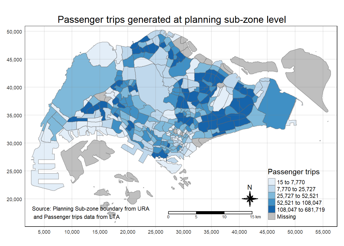
:::